38 excel pivot table 2 row labels
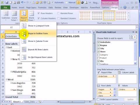
Customizing a pivot table | Microsoft Press Store The Excel team added the Repeat All Item Labels option to the Report Layout tab starting in Excel 2010. This alleviated a lot of busy work because it takes just two clicks to fill in all the blank cells along the outer row fields. ... This setting applies only to pivot tables with two or more row fields. Blank rows are not added after each item ... Two columns of headers, want to show up in one row of pivot table Re: Two columns of headers, want to show up in one row of pivot table. If you are willing to use Power Query/Get and Transform then this can be achieved without a pivot table. Group your data in the Power Query Editor. Please Login or Register to view this content. Duplicate the table and remove all steps to create a new query.
Excel: How to Filter Data in Pivot Table Using "Greater Than" To do so, click the dropdown arrow next to Row Labels, then click Value Filters, then click Greater Than: In the window that appears, type 10 in the blank space and then click OK: The pivot table will automatically be filtered to only show rows where the Sum of Sales is greater than 10: To remove the filter, simply click the dropdown arrow next ...

Excel pivot table 2 row labels
rename row labels in pivot table - authoreminence.com May 11, 2022 May 11, 2022 contigo spill-proof straw replacement. rename row labels in pivot table PivotTable.DataLabelRange property (Excel) | Microsoft Docs In this article. Returns a Range object that represents the range that contains the labels for the data fields in the PivotTable report. Read-only. Syntax. expression.DataLabelRange. expression A variable that represents a PivotTable object.. Example. This example selects the data field labels in the PivotTable report. Excel: How to Sort Pivot Table by Date - Statology Before creating a pivot table for this data, click on one of the cells in the Date column and make sure that Excel recognizes the cell as a Date format: Next, we can highlight the cell range A1:B10, then click the Insert tab along the top ribbon, then click PivotTable, and insert the following pivot table to summarize the total sales for each ...
Excel pivot table 2 row labels. Excel Pivot Table Filter and Label Formatting - Microsoft Tech Community Excel 2016. Images of 2 separate workbooks, each with a data table, pivot table and pivot chart, the one on the right created by copy & paste of the one on the left. The one on the right changed: X axis labels on the pivot chart don't have the multi-level option. Also, unlike the original on the left, there is now a filter button for the chart. How To Add Data Labels In Excel Guide 2022 - IND4 Blog Take a good look at your excel worksheet. Click add data label, then click add data callout. Source: hima4.cdtla.org. To format data labels, select your chart, and then in the chart design tab, click add chart element > data labels > more data label options. The result is that your data label will appear in a graphical. Solved: Pivot Table with multiple same values - Power BI Hi all, May I seek any help for this table transform? ID Name Value 1 Category Shipment 1 Item A 1 Price 100 1 Item B 1 Price 200 1 Item C 2 Category Delivery 2 Item A 2 Price 150 Desired Output: ID Category Item Price 1 Shipment A 100 1 Shipment B 200 1 Shipment C 2 Delivery A 150 Appreciated... Dimensions and Measures in Excel Pivot Tables - Windsong Training Fig. 1: The name of an Excel table is on the Table Design contextual tab. To insert a pivot table for the current data set, click on a cell in the table, or select the entire table, and go the Insert tab -> Tables group. Click the PivotTable down arrow and select From Table/Range as shown in Fig. 2.
Excel Pivot Table tutorial - Ablebits 2. Create a pivot table. Select any cell in the source data table, and then go to the Insert tab > Tables group > PivotTable. This will open the Create PivotTable window. Make sure the correct table or range of cells is highlighted in the Table/Range field. Then choose the target location for your Excel pivot table: stackoverflow.com › questions › 21940443Excel pivot table - average of calculated sums - Stack Overflow As a workaround you can use another pivot table, which takes the input as the original pivot table to find the average. pivot tables. The second pivot table has data source as- E3:F5 or till whatever row you require. You'll have to refresh all so that the second pivot table reflects any changes in the filter of first pivot table. Excel pivot table shows only when rows have multiple other types of ... I would like to use pivot table to show only rows which have another type of rows more than two rows. Over here, first (4 rows) and third (2 rows) row labels have more than two another rows. I would . Stack Overflow. About; Products For Teams; Stack Overflow ... › excel-pivot-table-formatHow to Format Excel Pivot Table - Contextures Excel Tips May 23, 2022 · Keep Formatting in Excel Pivot Table. A pivot table is automatically formatted with a default style when you create it, and you can select a different style later, or add your own formatting. For example, in the pivot table shown below, colour has been added to the subtotal rows, and column B is narrow.
en.wikipedia.org › wiki › Pivot_tablePivot table - Wikipedia Row labels are used to apply a filter to one or more rows that have to be shown in the pivot table. For instance, if the "Salesperson" field is dragged on this area then the other output table constructed will have values from the column "Salesperson", i.e. , one will have a number of rows equal to the number of "Sales Person". 【Excel 2016 の基本】ピボットテーブルの行ラベルを並べ替えるには? | ザイタクの心得 Excel で、ピボットテーブルを作成したあと、テーブル内の任意の行ラベルを移動させたいと思うことはないだろうか。今回は、ピボットテーブルのの行ラベルを並べ替える方法を紹介したい。※ピボットテーブルの作成方法は、以下を参照。ピボットテーブル How To Create A Pivot Table In Excel - Naukri Learning Step 1 - Insert your data on the excel sheet. Click any cell in the source data and go to the Insert tab. Click the PivotTable button inside the Tables group. You can also choose the Recommended PivotTables option to check for other options. Excel offers other previews to insert your dynamic periodic table. PivotTable with Multiple Text Values Alternative - Excel University Pivot Column. We select the entire Return column, and select Transform > Pivot Column. In the resulting Pivot Column dialog, we select StaffList as the Values Column. We then expand the Advanced options and select Don't Aggregate (or Minimum or Maximum): We hit OK, and bam: Finally, we can send the results to Excel.
Multiple Row Fields
How to Use Excel Pivot Table Label Filters Watch the steps in this short video, and the written instructions are below the video. Play. To change the Pivot Table option to allow multiple filters: Right-click a cell in the pivot table, and click PivotTable Options. Click the Totals & Filters tab Under Filters, add a check mark to 'Allow multiple filters per field.'.

Design your Pivot Table in Excel | Excel in Excel
How to Filter Excel Pivot Table (8 Effective Ways) - ExcelDemy Furthermore, you can filter the whole Pivot Table by specifying a value. Suppose, you want to get the sum of sales that is greater than 2500. ⏩ Click on the drop-down arrow of Row Labels. ⏩ Go to Value Filters > Greater Than. ⏩ And now, put the specified value in the box that is 2500 and press OK.

Pivot table row labels in separate columns • AuditExcel.co.za
Repeat Pivot Table row labels - AuditExcel.co.za How to repeat the row labels. So to repeat pivot table row labels, you can right click in the column where you want the row labels repeated and click on Field Settings as shown below. In the Field Settings box you need to click on the Layout & Print tab and choose the 'Repeat items labels'. Like magic you will now see the row labels ...

Excel pivot table hides complete row when blank values or labels are filtered - Super User
Consolidate Multiple Worksheets into Excel Pivot Tables Consolidate Multiple Worksheets using the Pivot Table Wizard. First press Alt+D, then press P. Excel displays the The Pivot Table Wizard dialog box. A summary of data tables before we consolidate the worksheets: Sames ranges, same shapes, and same labels are required to combine datasets into a pivot table. Now check the Multiple consolidation ...

How to Sort Data in a Pivot Table | Excelchat
How to Transpose a Table in Excel (5 Suitable Methods) Method 3: Use Pivot Table to Transpose a Table in Excel. In this method, I will use the Pivot Table to Transpose the data. It is pretty lengthy but simple. Step 1: Select the whole table. Go to Insert menu ribbon Pick the Pivot Table option. A box will pop up.

Excel Pivot Table Report - Sort Data in Row & Column Labels & in Values Area, use Custom Lists
excel - Shifting Row Sub label to another column in Pivot Table - Stack ... 1. If you are OK with having the country in Column 2, merely change the Report Layout to show in tabular form and you may also want to do not show subtotals. - Ron Rosenfeld. Oct 25 '21 at 13:44. Add a comment.

Excel Help: Simple method to make Pivot table
How to Remove Old Row and Column Items from the Pivot Table in Excel? Following are the steps: Step 1: Right-click inside any cell of the pivot table. For example, right-click inside cell C6, cell value Arushi. A drop-down appears. Click on the refresh button. Step 2: PivotTable Options dialogue box appears. Go to the Data tab. Under, Retain items deleted from the data source section, go to Number of items to ...

How to Use Excel in 2017: 14 Simple Excel Shortcuts, Tips & Tricks
Filter by Labels - Text | MyExcelOnline STEP 1: Click on the Row Label filter button in the Pivot Table. STEP 2: Select Label Filters. You will see that we have a lot of filtering options. Let us try out - Ends With. STEP 3: Type in ber to get the months ending in ber. You can see that the Label Filter will be applied to the SALES MONTH. Click OK.
How to use a pivot table in Excel 2013 - Quora
› blog › insert-blank-rows-inHow to Insert a Blank Row in Excel Pivot Table - MyExcelOnline Jan 17, 2021 · Pivot Table reports are shown in a Compact Layout format as a default and if you have two or more Items in the Row Labels (e.g.Month & Customer), then the Pivot Table report can look very clunky… There is a cool little trick that most Excel users do not know about that adds a blank row after each item, making the Pivot Table report look more ...

23 things you should know about Excel pivot tables | Exceljet
How to Move Excel Pivot Table Labels Quick Tricks Use Menu Commands to Move Label. To move a pivot table label to a different position in the list, you can use commands in the right-click menu: Right-click on the label that you want to move. Click the Move command. Click one of the Move subcommands, such as Move [item name] Up. The existing labels shift down, and the moved label takes its new ...

Pivot Table in Microsoft Excel - Pivot Table Field List Report Functions of Filter Column Labels ...
powerspreadsheets.com › excel-pivot-table-groupExcel Pivot Table Group: Step-By-Step Tutorial To Group Or ... In fact, as mentioned in Excel 2016 Pivot Table Data Crunching: Each time you create a new pivot table in Excel 2016, Excel automatically shares the pivot cache. Pivot Cache sharing has several benefits. Most notably, as I mention above, it reduces memory requirements and file size vs. the scenario where the Pivot Cache isn't shared.

Remove Group Heading Excel Pivot Table - Stack Overflow
Sorting Row Labels in a Pivot Table by Month - Microsoft Community I have a column using the =TEXT (A1,"mmm-yy") to get them grouped by month. I thine put that column in a pivot table but the table doesn't go from January -December. It does it by the first letter so April, Aug, Feb etc., Can you help me to get it sorted, Jan, Feb, Mar, Apr, May, June etc etc. Thank you in advance. This thread is locked.
Repeat Headings in Excel 2010 Pivot Table - YouTube
Print Excel Pivot Table on two pages | MyExcelOnline Go to PivotTable Analyze > Actions > Select > Entire PivotTable. STEP 2: Go to Page Layout > Page Setup > Print Area > Set Print Area. Our print area based on our Pivot Table is now set. STEP 3: Select the 2014 row then go to Page Layout > Page Setup > Breaks > Insert Page Break. STEP 4: Now with our page break all set, go to PivotTable Analyze ...
Create a Pivot Table in Excel - The Complete Beginners Guide - QuickExcel
Pivot Table "Row Labels" Header Frustration - Microsoft Tech Community Enabling Remote Work. Small and Medium Business. Humans of IT. Empowering technologists to achieve more by humanizing tech. Green Tech. Raise awareness about sustainability in the tech sector. MVP Award Program. Find out more about the Microsoft MVP Award Program.

How to reset a custom pivot table row label
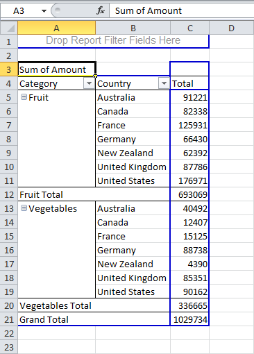
› excel-pivot-table-subtotalsExcel Pivot Table Subtotals - Contextures Excel Tips Feb 01, 2022 · In the pivot table shown below, Service is in the Row Labels area, Lead Tech is in the Column Labels area, and Labor Cost is in the Values area. Because Service is the only field in the Row Labels area, it has no subtotal. Multiple Row Fields. When you add another field to the Row Labels area, a subtotal is automatically created for the first ...
Why pivot table doesn't sort properly row labels? : excel
chandoo.org › wp › quick-tip-rename-headers-in-pivotQuick tip: Rename headers in pivot table so they are presentable Mar 15, 2018 · Pivot tables are fun, easy and super useful. Except, they can be ugly when it comes to presentation. Here is a quick way to make a pivot look more like a report. Just type over the headers / total fields to make them user friendly. See this quick demo to understand what I mean: So simple and effective.

Can I use the union of two columns values in Excel as row labels in a Pivot Table? - Super User
PivotTable.MergeLabels property (Excel) | Microsoft Docs In this article. True if the specified PivotTable report's outer-row item, column item, subtotal, and grand total labels use merged cells. Read/write Boolean.. Syntax. expression.MergeLabels. expression A variable that represents a PivotTable object.. Example. This example causes the first PivotTable report on worksheet one to use merged-cell outer-row item, column item, subtotal, and grand ...
Post a Comment for "38 excel pivot table 2 row labels"