42 excel pivot table column labels
Filtering Grand Total Amounts Within Excel Pivot Tables Click the arrow in the Column Labels field. Uncheck the checkboxes for all items except Apples and Oranges. Click OK. The pivot table only displays columns for Apples and Oranges. Figure 3: The pivot table allows you to filter for specific columns. You can filter rows in a similar fashion, as shown in Figure 4: Click the arrow in the Row Labels ... Excel Pivot Table Report - Clear All, Remove Filters, Select … Pivot Table Options tab - Actions group Customizing a Pivot Table report: When you insert a Pivot Table, a blank Pivot Table report is created in the specified location, and the 'PivotTable Field List' Pane also appears which allows you to Add or Remove Fields, Move Fields to different Areas and to set Field Settings. The 'Options' and 'Design' tabs (under the 'PivotTable Tools' …
How to Customize Your Excel Pivot Chart Data Labels - dummies The Data Labels command on the Design tab's Add Chart Element menu in Excel allows you to label data markers with values from your pivot table. When you click the command button, Excel displays a menu with commands corresponding to locations for the data labels: None, Center, Left, Right, Above, and Below.

Excel pivot table column labels
Excel Pivot Table Subtotals - Contextures Excel Tips Feb 01, 2022 · Creating Pivot Table Subtotals . If your pivot table has only one field in the Row Labels area, you won't see any Row subtotals. In the pivot table shown below, Service is in the Row Labels area, Lead Tech is in the Column Labels area, and Labor Cost is in the Values area. Hide Pivot Table Buttons and Labels - Contextures Blog Right-click a cell in the pivot table and, in the pop up menu, click PivotTable Options. In the Display section, remove the check mark from Show Expand/Collapse Buttons. This change will hide the Expand/Collapse buttons to the left of the outer Row Labels and Column Labels. Next, remove the check mark from Display Field Captions and Filter Drop ... Changing Blank Row Labels - Excel Pivot Tables Select one of the Row or Column Labels that contains the text (blank). Type N/A in the cell, and then press the Enter key. Note: All other (Blank) items in that field will change to display the same text, N/A in this example. For more information on pivot tables, see the Pivot Table Topics on my Contextures web site.
Excel pivot table column labels. How to group time by hour in an Excel pivot table? (3) Specify the location you will place the new pivot table. 3. Click the Ok button. 4. Then a pivot table is created with a Half an hour column added as rows. Go ahead to add the Amount column as values. So far, the pivot table has been created based on the selection, and data has been grouped by half an hour as above screenshot shown. How to Create Excel Pivot Table [Includes practice file] 15-01-2022 · One different area is the pivot table has its own options. You can use these options by right-clicking a cell within and selecting PivotTable Options… For example, you might only want Grand Totals for columns and not rows. There are also ways to filter the data using the controls next to Row Labels or Column labels on the pivot table. How to insert a blank column in pivot table? - Chandoo.org 16-04-2015 · We all know pivot table functionality is a powerful & useful feature. But it comes with some quirks. For example, we cant insert a blank row or column inside pivot tables. So today let me share a few ideas on how you can insert a blank column. But first let's try inserting a column Imagine you are looking at a pivot table like above. And you want to insert a column or row. … Excel Pivot Table Subtotals - Contextures Excel Tips 01-02-2022 · Creating Pivot Table Subtotals . If your pivot table has only one field in the Row Labels area, you won't see any Row subtotals. In the pivot table shown below, Service is in the Row Labels area, Lead Tech is in the Column Labels area, and …
How to rename group or row labels in Excel PivotTable? 1. Click at the PivotTable, then click Analyze tab and go to the Active Field textbox. 2. Now in the Active Field textbox, the active field name is displayed, you can change it in the textbox. You can change other Row Labels name by clicking the relative fields in the PivotTable, then rename it in the Active Field textbox. How to Use Excel Pivot Table Label Filters Right-click a cell in the pivot table, and click PivotTable Options. Click the Totals & Filters tab Under Filters, add a check mark to 'Allow multiple filters per field.' Click OK Quick Way to Hide or Show Pivot Items Easily hide or show pivot table items, with the quick tip in this video. The written instructions are below the video Change Blank Labels in a Pivot Table - Contextures Blog You can type any text to replace the (Blank) entry, even a space character, but you can't clear the cell and leave it empty: Select one of the Row or Column Labels that contains the text (blank). Type N/A in the cell, and then press the Enter key. Note: All other (Blank) items in that field will change to display the same text, N/A in this ... How to Add a Column to a Pivot Table - Excel Tutorials Add a Column to a Pivot Table. Now that we have our data into the Pivot Table, we will put players into the row field and averages of points into the value fields: If you, for whatever reason, wanted a different value (for example, a total sum of points) all you have to do is click the field in values (in this case Average of Points) and select ...
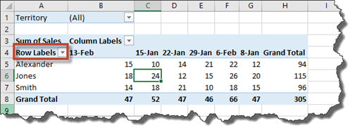
Combining Column Values in an Excel Pivot Table - Stack Overflow In your pivot table, Select the Pivot Table Tools> Analyze tab, then "Fields, Items",then pull down to"Calculated fields". Enter a name for the generated field, and the formula you want to use: In my example, I added the fields Fruit and Vegi's from my available pivot table fields (which is based on my data table). Remove PivotTable Duplicate Row Labels - Excel Help Forum Re: Remove PivotTable Duplicate Row Labels. Sometimes when the cells are stored in different formats within the same column in the raw data, they get duplicated. Also, if there is space/s at the beginning or at the end of these fields, when you filter them out they look the same, however, when you plot a Pivot Table, they appear as separate ... How to Create a Pivot Table in Excel: A Step-by-Step Tutorial 31-12-2021 · Every pivot table in Excel starts with a basic Excel table, where all your data is housed. To create this table, simply enter your values into a specific set of rows and columns. Use the topmost row or the topmost column to categorize your values by what they represent. Excel tutorial: How to filter a pivot table by rows or columns When you add a field as a row or column label in a pivot table, you automatically get the ability to filter the results in the table by items that appear in that field. Let's take a look. This pivot table is displaying just one field: Total Sales. After we add Product as a row label, notice that a drop-down arrow appears in the header area.

Multi-level Pivot Table in Excel - EASY Excel Tutorial
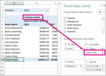
Excel tutorial: How to rename fields in a pivot table Either right-click on the field and choose Value field settings, or click Field Settings on the Options Tab of the PivotTable Tools ribbon. Here, you can see the original field name. In contrast to value fields, Row and Column label field names will be identical to the name in the field list. In fact, they are linked, as we'll see in a minute.

Use column labels from an Excel table as the rows in a Pivot Table - Stack Overflow
Design the layout and format of a PivotTable In the PivotTable, right-click the row or column label or the item in a label, point to Move, and then use one of the commands on the Move menu to move the item to another location. Select the row or column label item that you want to move, and then point to the bottom border of the cell.

Introduction To Pivot Table – Excel Tutorial World
Combining Column Values in an Excel Pivot Table - Stack Overflow In order to simplify a stacked bar chart, I am looking to sum up the counts of multiple columns I have in my pivot table. For example, in this sample table, I would like to combine Fruits and Vegetables into one column, so that each bar will comprised of three colors: one for Meats, one for Grains, and one for Fruits+Vegetables.

excel - Pivot Table shows blank value labels - Stack Overflow
Pivot table row labels in separate columns • AuditExcel.co.za Our preference is rather that the pivot tables are shown in tabular form (all columns separated and next to each other). You can do this by changing the report format. So when you click in the Pivot Table and click on the DESIGN tab one of the options is the Report Layout. Click on this and change it to Tabular form.
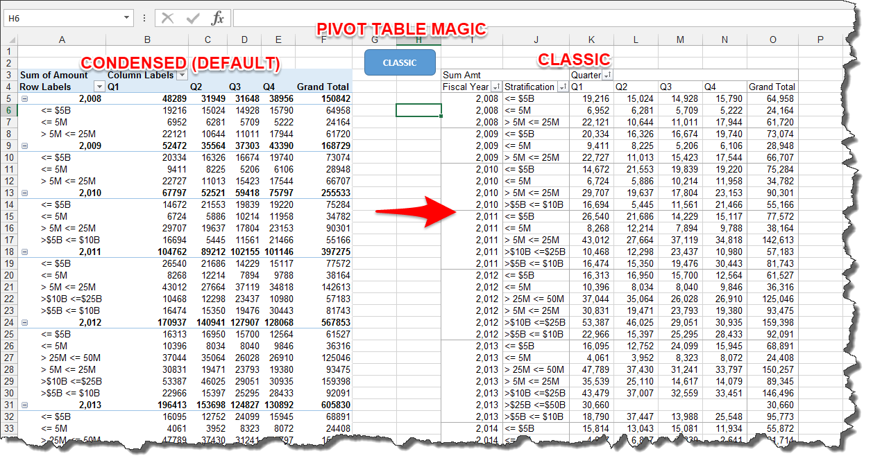
Microsoft Excel — Pivot Table Magic – Let’s Excel – Medium
How to Move Excel Pivot Table Labels Quick Tricks To move a pivot table label to a different position in the list, you can use commands in the right-click menu: Right-click on the label that you want to move Click the Move command Click one of the Move subcommands, such as Move [item name] Up The existing labels shift down, and the moved label takes its new position. Type Over Another Label

31 How To Label Excel Columns - Labels Database 2020
Format column labels in pivot table | MrExcel Message Board Move the field to row labels. Point to the top edge of the field button until the pointer changes to , and then click. Format it and move it back to column labels You must log in or register to reply here. Similar threads VBA to Filter Column Labels of a Pivot Table SanjayGulatiMusafir Nov 25, 2021 Excel Questions Replies 0 Views 204 Nov 25, 2021

Excel Pivot Table Report - Sort Data in Row & Column Labels & in Values Area, use Custom Lists
How to Move Excel Pivot Table Labels Quick Tricks 12-07-2021 · Move Pivot Table Labels. This short video shows 3 ways to manually move the labels in a pivot table, and the written instructions are below the video. Drag a Label. Use Menu Commands. Type over a Label. Drag Labels to New Position. To move a pivot table label to a different position in the list, you can drag it:
Discover Pivot Tables – Excel’s most powerful feature and also least known
Use column labels from an Excel table as the rows in a Pivot Table Highlight your current table, including the headers Then from the Data section of the ribbon, select From Table Highlight all the columns containing data, but not the Year column, and then select Unpivot Columns Close the dialog and keep the changes. Excel should place the unpivoted data into a new worksheet, looking something like this:

Pivot table row labels in separate columns • AuditExcel.co.za
Automatic Row And Column Pivot Table Labels - How To Excel At Excel Select the data set you want to use for your table The first thing to do is put your cursor somewhere in your data list Select the Insert Tab Hit Pivot Table icon Next select Pivot Table option Select a table or range option Select to put your Table on a New Worksheet or on the current one, for this tutorial select the first option Click Ok
MS Excel 2013: Display the fields in the Values Section in multiple columns in a pivot table
Filter Excel pivot table using VBA - Stack Overflow PvtTbl.ManualUpdate = True 'Adds row and columns for pivot table PvtTbl.AddFields RowFields:="VerifyHr", ColumnFields:=Array("WardClinic_Category", "IVUDDCIndicator") 'Add item to the Report Filter PvtTbl.PivotFields("DayOfWeek").Orientation = xlPageField 'set data field - specifically change orientation to a data field and set its function ...

How to Add Rows to a Pivot Table: 10 Steps (with Pictures)
How to group time by hour in an Excel pivot table? (3) Specify the location you will place the new pivot table. 3. Click the Ok button. 4. Then a pivot table is created with a Half an hour column added as rows. Go ahead to add the Amount column as values. So far, the pivot table has been created based on the selection, and data has been grouped by half an hour as above screenshot shown.

Design your Pivot Table in Excel | Excel in Excel
How to make row labels on same line in pivot table? Make row labels on same line with PivotTable Options You can also go to the PivotTable Options dialog box to set an option to finish this operation. 1. Click any one cell in the pivot table, and right click to choose PivotTable Options, see screenshot: 2.
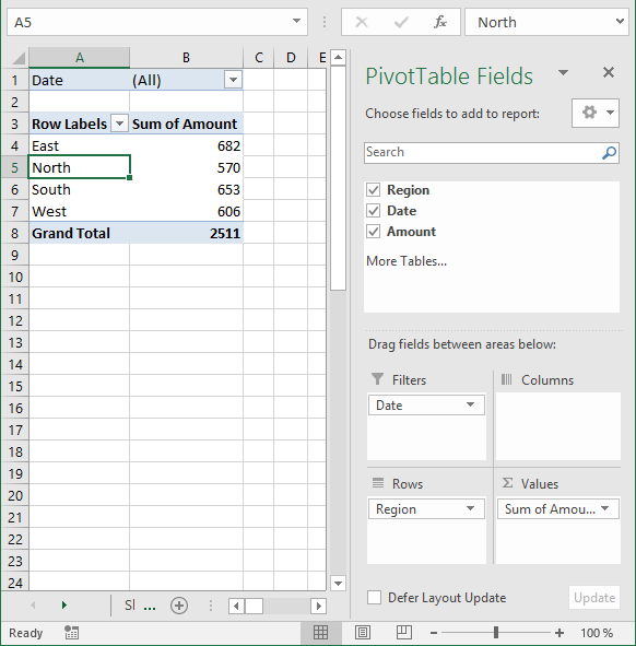
Use the Field List to arrange fields in a PivotTable in Excel 2016 for Windows - Excel
How to reverse a pivot table in Excel? - ExtendOffice Reverse pivot table with Kutools for Excel’s Transpose Table Dimensions. With above way, there are so many steps to solve the task. ... Click OK, and in PivotTable Field List pane, drag Row and Column fields to Row Labels section, and Value field to Values section. 6.

How To Make Awesome Ranking Charts With Excel Pivot Tables - Moz
Spreadsheets: Problems with Pivot Table Labels - CFO To return to a normal layout of the pivot table, follow these steps: 1. Select any cell inside the pivot table. The PivotTable Tools tabs appear in the Ribbon. 2. Go to Design tab of the ribbon. 3. From the Design tab, open the Report Layout dropdown. 4.
Using Pivot Tables in Excel 2016 | UniversalClass
How to reverse a pivot table in Excel? - ExtendOffice 5. Now a new pivot table is created, and double click last cell at the right down corner of new Pivot table, then a new table is created in a new worksheet. See screenshots: iv> 6. Then create a new pivot table based on this new table. Select the whole new table, and click Insert > PivotTable > PivotTable. 7.

How to Sort Pivot Table Row Labels, Column Field Labels and Data Values with Excel VBA Macro ...
How to add column labels in pivot table [SOLVED] Re: How to add column labels in pivot table Here are the steps 1. Add a helper column showing Month Text Just as I have done in Column H 2. Now insert a Pivot Table 3. Put Fields in there required sections in the Pivot table Field List Window just as I have done . 4.
Post a Comment for "42 excel pivot table column labels"