40 excel chart custom data labels
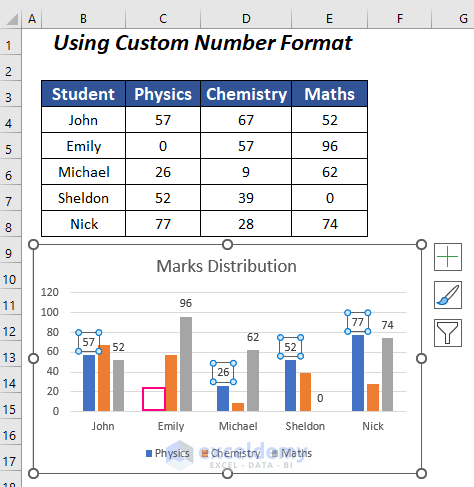
Remove Chart Data Labels With Specific Value The two methodologies covered are: Utilizing Custom Number Format rules Deleting the Data Label Remove Data Labels Equal To Zero Hide Zeroes With Custom Number Format Rule This VBA code modifies the custom number format rule for the selected chart's data labels so that zero values are hidden. Sub RemoveDataLabels_ByNumberFormat () support.microsoft.com › en-us › officeAdd or remove data labels in a chart - support.microsoft.com You can add data labels to show the data point values from the Excel sheet in the chart. This step applies to Word for Mac only: On the View menu, click Print Layout . Click the chart, and then click the Chart Design tab.
How to Display Percentage in an Excel Graph (3 Methods) Display Percentage in Graph. Select the Helper columns and click on the plus icon. Then go to the More Options via the right arrow beside the Data Labels. Select Chart on the Format Data Labels dialog box. Uncheck the Value option. Check the Value From Cells option.

Excel chart custom data labels
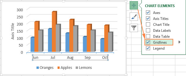
How to format axis labels individually in Excel - SpreadsheetWeb How to add custom formatting to a chart's axis Double-click on the axis you want to format. Double-clicking opens the right panel where you can format your axis. Open the Axis Options section if it isn't active. You can find the number formatting selection under Number section. Select Custom item in the Category list. How to set multiple series labels at once - Microsoft Tech Community Click anywhere in the chart. On the Chart Design tab of the ribbon, in the Data group, click Select Data. Click in the 'Chart data range' box. Select the range containing both the series names and the series values. Click OK. If this doesn't work, press Ctrl+Z to undo the change. 0 Likes Reply Nathan1123130 replied to Hans Vogelaar How to Add Two Data Labels in Excel Chart (with Easy Steps) Select the data labels. Then right-click your mouse to bring the menu. Format Data Labels side-bar will appear. You will see many options available there. Check Category Name. Your chart will look like this. Now you can see the category and value in data labels. Read More: How to Format Data Labels in Excel (with Easy Steps) Things to Remember
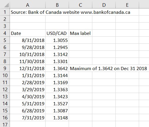
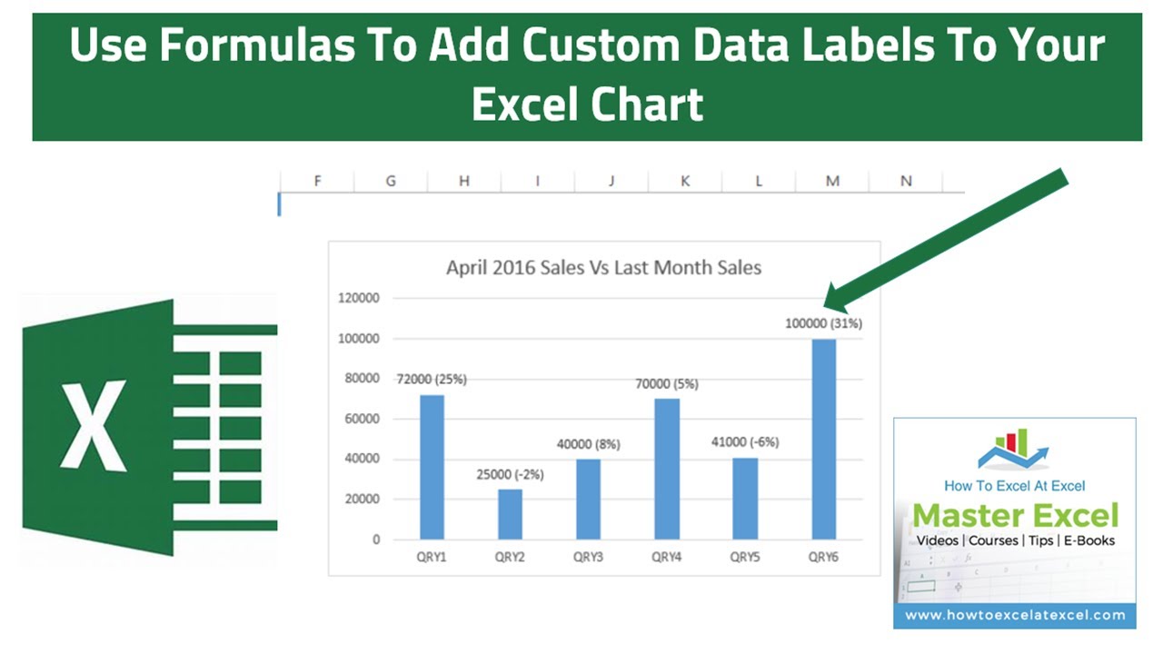
Excel chart custom data labels. Create Custom Data Labels. Excel Charting. In this video, we'll show you how to add custom data labels using formulas. We'll also provide some tips on how to make sure your data labels look great on your chart. So, today let's have a look at using a few types of formulas to add some really cool custom data labels to our Excel charts. data labels in excel - temp.lovelysheetworkideas.co How to Change Excel Chart Data Labels to Custom Values?. Quick Tip: Excel 2013 offers flexible data labels - TechRepublic. How to Add Data Labels to an Excel 2010 Chart - dummies. Adding rich data labels to charts in Excel 2013 - Microsoft 365 Blog. support.microsoft.com › en-us › officeChange the format of data labels in a chart To get there, after adding your data labels, select the data label to format, and then click Chart Elements > Data Labels > More Options. To go to the appropriate area, click one of the four icons ( Fill & Line , Effects , Size & Properties ( Layout & Properties in Outlook or Word), or Label Options ) shown here. Excel Charts Creating Custom Data Labels - Otosection Surface Studio vs iMac - Which Should You Pick? 5 Ways to Connect Wireless Headphones to TV. Design
Data Labels in Excel Pivot Chart (Detailed Analysis) 7 Suitable Examples with Data Labels in Excel Pivot Chart Considering All Factors 1. Adding Data Labels in Pivot Chart 2. Set Cell Values as Data Labels 3. Showing Percentages as Data Labels 4. Changing Appearance of Pivot Chart Labels 5. Changing Background of Data Labels 6. Dynamic Pivot Chart Data Labels with Slicers 7. Chart data labels and CAGR arrows - UpSlide Help & Support Select the data series which contains the label you want Choose Select a Single Label and in the dropdown choose the data point you want to apply a custom position to Enter the number of points you want the labels to move by and then press the arrow for the direction of movement Close the window to see the effect on the chart DataLabels object (Excel) | Microsoft Learn Example Use the DataLabels method of the Series object to return the DataLabels collection. The following example sets the number format for data labels on series one on chart sheet one. VB With Charts (1).SeriesCollection (1) .HasDataLabels = True .DataLabels.NumberFormat = "##.##" End With DataLabels collection (Excel Graph) | Microsoft Learn In this article. A collection of all the DataLabel objects for the specified series. Each DataLabel object represents a data label for a point or trendline. For a series without definable points (such as an area series), the DataLabels collection contains a single data label.. Remarks. Use the DataLabels method to return the DataLabels collection.. Use DataLabels (index), where index is the ...
› make-labels-with-excel-4157653How to Print Labels from Excel - Lifewire Apr 05, 2022 · How to Print Labels From Excel . You can print mailing labels from Excel in a matter of minutes using the mail merge feature in Word. With neat columns and rows, sorting abilities, and data entry features, Excel might be the perfect application for entering and storing information like contact lists. How to add text labels on Excel scatter chart axis - Data Cornering 3. Add dummy series to the scatter plot and add data labels. 4. Select recently added labels and press Ctrl + 1 to edit them. Add custom data labels from the column "X axis labels". Use "Values from Cells" like in this other post and remove values related to the actual dummy series. Change the label position below data points. Adding Data Labels to Your Chart (Microsoft Excel) - ExcelTips (ribbon) To add data labels in Excel 2013 or later versions, follow these steps: Activate the chart by clicking on it, if necessary. Make sure the Design tab of the ribbon is displayed. (This will appear when the chart is selected.) Click the Add Chart Element drop-down list. Select the Data Labels tool. Pie Chart in Excel - Inserting, Formatting, Filters, Data Labels Click on the Instagram slice of the pie chart to select the instagram. Go to format tab. (optional step) In the Current Selection group, choose data series "hours". This will select all the slices of pie chart. Click on Format Selection Button. As a result, the Format Data Point pane opens.
Is there a way to show different data labels in a bar chart ...
› 509290 › how-to-use-cell-valuesHow to Use Cell Values for Excel Chart Labels - How-To Geek Mar 12, 2020 · Select the chart, choose the “Chart Elements” option, click the “Data Labels” arrow, and then “More Options.” Uncheck the “Value” box and check the “Value From Cells” box. Select cells C2:C6 to use for the data label range and then click the “OK” button.

Change axis labels in a chart
DataLabel object (Excel) | Microsoft Learn Use the DataLabel property of the Point object to return the DataLabel object for a single point. The following example turns on the data label for the second point in series one on the chart sheet named Chart1, and sets the data label text to Saturday. On a trendline, the DataLabel property returns the text shown with the trendline.
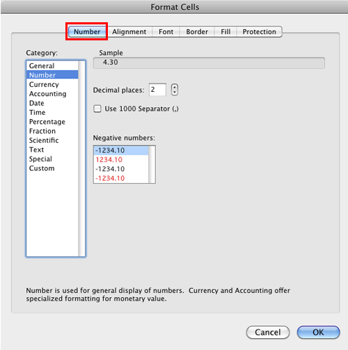
Format Number Options for Chart Data Labels in Excel 2011 for Mac
› how-to-create-excel-pie-chartsHow to Make a Pie Chart in Excel & Add Rich Data Labels to ... Sep 08, 2022 · In this article, we are going to see a detailed description of how to make a pie chart in excel. One can easily create a pie chart and add rich data labels, to one’s pie chart in Excel. So, let’s see how to effectively use a pie chart and add rich data labels to your chart, in order to present data, using a simple tennis related example.

Add or remove data labels in a chart
How to Add Data Labels to Scatter Plot in Excel (2 Easy Ways) - ExcelDemy 2 Methods to Add Data Labels to Scatter Plot in Excel 1. Using Chart Elements Options to Add Data Labels to Scatter Chart in Excel 2. Applying VBA Code to Add Data Labels to Scatter Plot in Excel How to Remove Data Labels 1. Using Add Chart Element 2. Pressing the Delete Key 3. Utilizing the Delete Option Conclusion Related Articles

Change the format of data labels in a chart
How do you label data points in Excel? - Profit claims 1. Right click the data series in the chart, and select Add Data Labels > Add Data Labels from the context menu to add data labels. 2. Click any data label to select all data labels, and then click the specified data label to select it only in the chart. 3.

How to Change Excel Chart Data Labels to Custom Values?
› documents › excelHow to rotate axis labels in chart in Excel? - ExtendOffice Rotate axis labels in Excel 2007/2010. 1. Right click at the axis you want to rotate its labels, select Format Axis from the context menu. See screenshot: 2. In the Format Axis dialog, click Alignment tab and go to the Text Layout section to select the direction you need from the list box of Text direction. See screenshot: 3.
Custom Axis Labels and Gridlines in an Excel Chart - Peltier Tech
Custom data labels pop-ups after hovering mouse over a scatter chart Currently with Excel charts I can have either (a) some information after mouse hovering or (b) custom data in my label but displayed constantly. a) hover label.png b) custom lavel.PNG The problem with both is that it'll be way too many data for a typical label, and the 'temporary label' seen after mouse hovering won't give me the data I need.

How to create Custom Data Labels in Excel Charts
DataLabels.Separator property (Excel) | Microsoft Learn This example sets the data label separator for the first series on the first chart to a semicolon. This example assumes that a chart exists on the active worksheet. VB Sub ChangeSeparator () ActiveSheet.ChartObjects (1).Chart.SeriesCollection (1) _ .DataLabels.Separator = ";" End Sub Support and feedback
Directly Labeling Excel Charts - PolicyViz
peltiertech.com › prevent-overlapping-data-labelsPrevent Overlapping Data Labels in Excel Charts - Peltier Tech May 24, 2021 · Overlapping Data Labels. Data labels are terribly tedious to apply to slope charts, since these labels have to be positioned to the left of the first point and to the right of the last point of each series. This means the labels have to be tediously selected one by one, even to apply “standard” alignments.

Apply Custom Data Labels to Charted Points - Peltier Tech
How to Add Two Data Labels in Excel Chart (with Easy Steps) Select the data labels. Then right-click your mouse to bring the menu. Format Data Labels side-bar will appear. You will see many options available there. Check Category Name. Your chart will look like this. Now you can see the category and value in data labels. Read More: How to Format Data Labels in Excel (with Easy Steps) Things to Remember
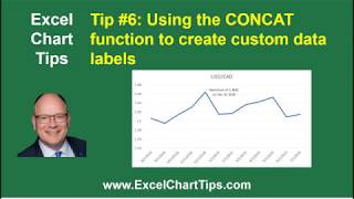
Using the CONCAT function to create custom data labels for an Excel chart
How to set multiple series labels at once - Microsoft Tech Community Click anywhere in the chart. On the Chart Design tab of the ribbon, in the Data group, click Select Data. Click in the 'Chart data range' box. Select the range containing both the series names and the series values. Click OK. If this doesn't work, press Ctrl+Z to undo the change. 0 Likes Reply Nathan1123130 replied to Hans Vogelaar

Add Custom Labels to x-y Scatter plot in Excel - DataScience ...
How to format axis labels individually in Excel - SpreadsheetWeb How to add custom formatting to a chart's axis Double-click on the axis you want to format. Double-clicking opens the right panel where you can format your axis. Open the Axis Options section if it isn't active. You can find the number formatting selection under Number section. Select Custom item in the Category list.
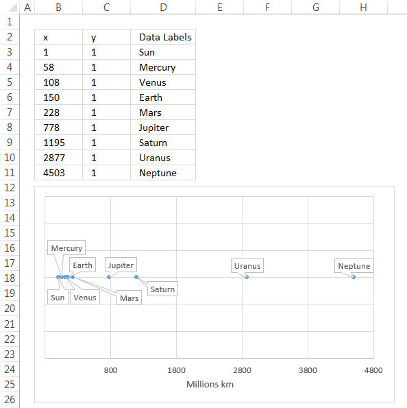
Improve your X Y Scatter Chart with custom data labels

Color Negative Chart Data Labels in Red with downward arrow
How to Remove Zero Data Labels in Excel Graph (3 Easy Ways)
microsoft excel - How do I reposition data labels with a ...
Working with Charts — XlsxWriter Documentation
Using the CONCAT function to create custom data labels for an ...

Google Workspace Updates: Get more control over chart data ...

Solved: How to show all detailed data labels of pie chart ...
Format Number Options for Chart Data Labels in Excel 2011 for Mac

Custom Data Labels with Colors and Symbols in Excel Charts ...

Color Negative Chart Data Labels in Red with downward arrow

Excel charts: add title, customize chart axis, legend and ...

Change the format of data labels in a chart
Add / Move Data Labels in Charts – Excel & Google Sheets ...

Apply Custom Data Labels to Charted Points - Peltier Tech

Change Horizontal Axis Values in Excel 2016 - AbsentData
vba - Excel XY Chart (Scatter plot) Data Label No Overlap ...

Change the format of data labels in a chart
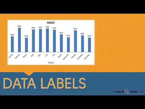
Adding Data Labels To An Excel Chart | MyExcelOnline

Apply Custom Data Labels to Charted Points - Peltier Tech
Excel charts: add title, customize chart axis, legend and ...
Using the CONCAT function to create custom data labels for an ...

Custom Excel Chart Label Positions • My Online Training Hub

Custom Data Labels with Colors and Symbols in Excel Charts ...

Adding rich data labels to charts in Excel 2013 | Microsoft ...

Change the format of data labels in a chart
Create Custom Data Labels. Excel Charting.

How-to Use Data Labels from a Range in an Excel Chart - Excel ...
Post a Comment for "40 excel chart custom data labels"