42 excel chart hide zero data labels
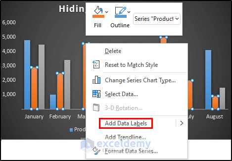
How to hide "0" in chart axis [quick tip] - Chandoo.org Have you ever wondered how you can hide that 0 (zero) at axis bottom? Like this…, Here is a handy little trick to do just that: Select the axis and press CTRL+1 (or right click and select "Format axis") Go to "Number" tab. Select "Custom". Specify the custom formatting code as #,##0;-#,##0;; Press "Add" if you are using Excel ... How to Add Two Data Labels in Excel Chart (with Easy Steps) How to Remove Zero Data Labels in Excel Graph (3 Easy Ways) Step 3: Apply 2nd Data Label in Excel Chart In this section, I will show how to apply another data label to this chart. Let's express the demand units this time. Select any column representing demand units. Then right-click your mouse to bring the menu. After that, select Add Data Labels.
How can I hide 0% value in data labels in an Excel Bar Chart The quick and easy way to accomplish this is to custom format your data label. Select a data label. Right click and select Format Data Labels; Choose the Number category in the Format Data Labels dialog box.

Excel chart hide zero data labels
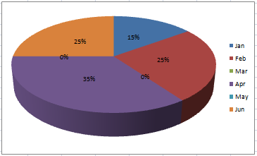
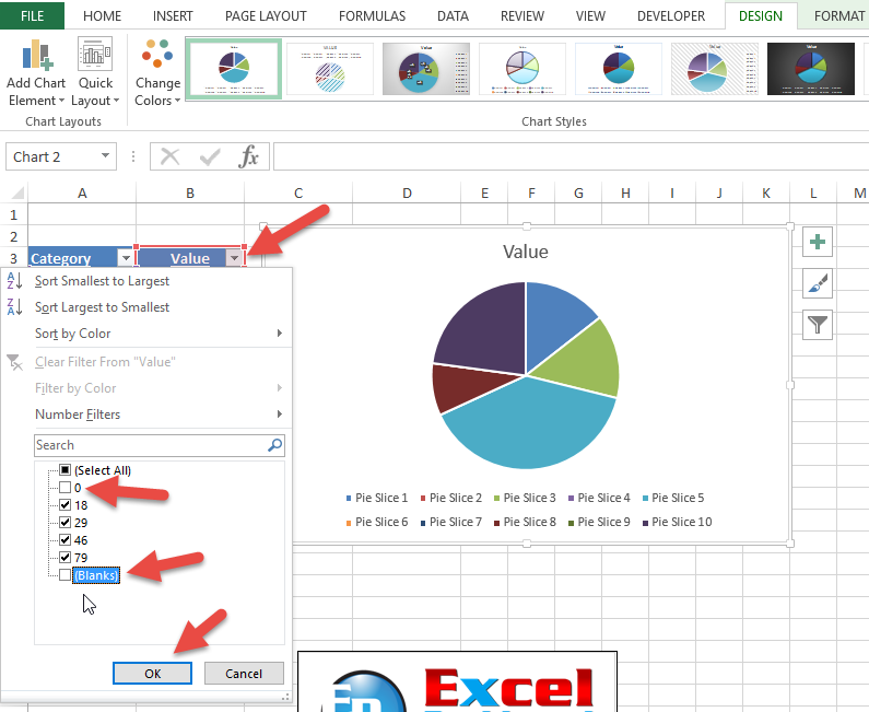
remove label with 0% in a pie chart. - social.msdn.microsoft.com Here is what I did: I wanted to remove the 0% percent labels from my pie chart that displays percentages next to each slice. Turn the range of cells that you want to make a pie chart with into a table. In excel 2007 you can do this by clicking Home>Format as Table>Select the Style You Want>Then Select the appropriate range. think-cell :: KB0195: How can I hide segment labels for If the chart is complex or the values will change in the future, an Excel data link (see Excel data links) can be used to automatically hide any labels when the value is zero ("0"). Open your data source Use cell references to read the source data and apply the Excel IF function to replace the value "0" by the text "Zero" Change the format of data labels in a chart To get there, after adding your data labels, select the data label to format, and then click Chart Elements > Data Labels > More Options. To go to the appropriate area, click one of the four icons ( Fill & Line, Effects, Size & Properties ( Layout & Properties in Outlook or Word), or Label Options) shown here.
Excel chart hide zero data labels. Hide Series Data Label if Value is Zero - Peltier Tech The trick is to use the value option for the data labels, rather than the series name option. The series names have been replaced by values, and zeros appear where the unwanted series name labels are in the chart above. Then apply custom number formats to show only the appropriate labels. Remove Chart Data Labels With Specific Value The two methodologies covered are: Utilizing Custom Number Format rules Deleting the Data Label Remove Data Labels Equal To Zero Hide Zeroes With Custom Number Format Rule This VBA code modifies the custom number format rule for the selected chart's data labels so that zero values are hidden. Sub RemoveDataLabels_ByNumberFormat () Column chart: Dynamic chart ignore empty values | Exceljet To make a dynamic chart that automatically skips empty values, you can use dynamic named ranges created with formulas. When a new value is added, the chart automatically expands to include the value. If a value is deleted, the chart automatically removes the label. In the chart shown, data is plotted in one series. Excel charts: add title, customize chart axis, legend and data labels Click the Chart Elements button, and select the Data Labels option. For example, this is how we can add labels to one of the data series in our Excel chart: For specific chart types, such as pie chart, you can also choose the labels location. For this, click the arrow next to Data Labels, and choose the option you want.
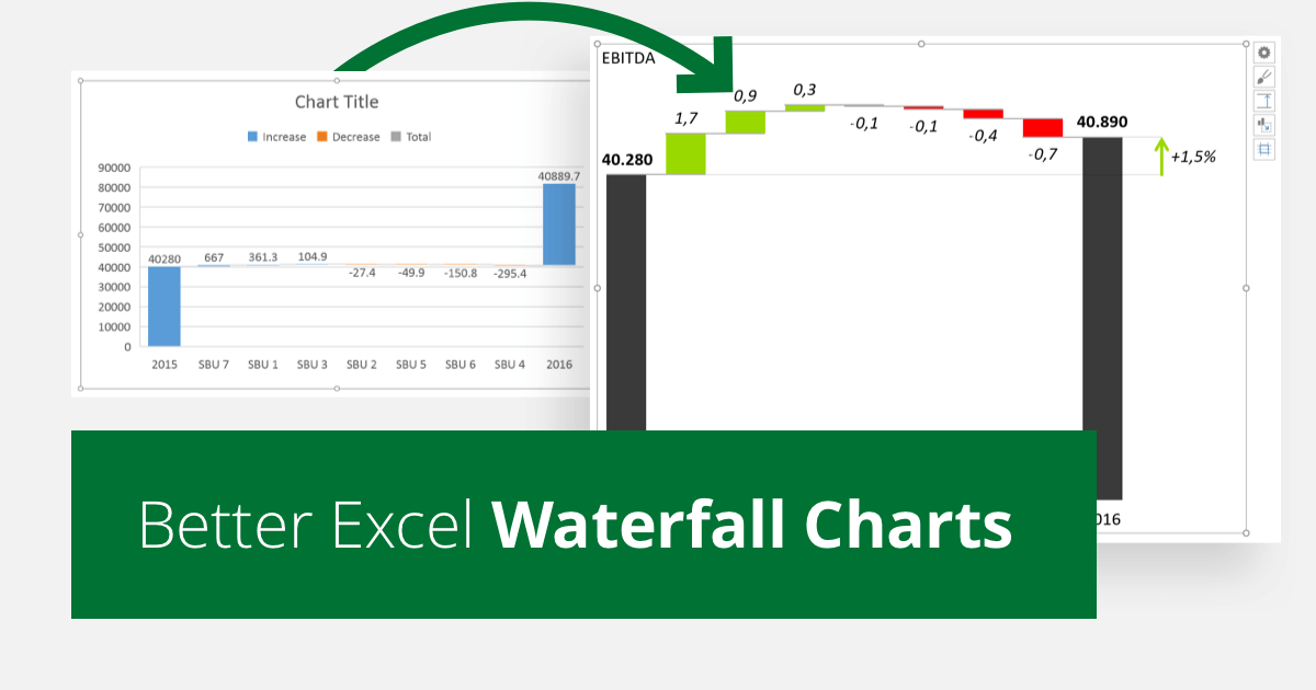
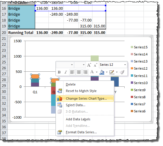
How can I hide 0-value data labels in an Excel Chart? Right click on a label and select Format Data Labels. Go to Number and select Custom. Enter #"" as the custom number format. Repeat for the other series labels. Zeros will now format as blank. NOTE This answer is based on Excel 2010, but should work in all versions Share Improve this answer edited Jun 12, 2020 at 13:48 Community Bot 1 › 07 › 25How to create waterfall chart in Excel - Ablebits.com Jul 25, 2014 · However, when you refer to the data table, you'll see that the represented values are different. For more accurate analysis I'd recommend to add data labels to the columns. Select the series that you want to label. Right-click and choose the Add Data Labels option from the context menu. Repeat the process for the other series. Hiding data labels with zero values | MrExcel Message Board Right click on a data label on the chart (which should select all of them in the series), select Format Data Labels, Number, Custom, then enter 0;;; in the Format Code box and click on Add. If your labels are percentages, enter 0%;;; or whatever format you want, with ;;; after it. With stacked column charts, you have to do this for each series ... Automatically eliminating zero-value data labels from charts I have a pie chart drawn from the following data: Item A: 10. Item B: 0 (in place as I might expect some value at a later time) Item C: 30. Item D: 60 . I did away with the legend in favor of data labels on each slice of the pie, showing percentages. So Excel generates: "Item A 10%" "Item B 0%" (along with a paper-thin slice of the pie) "Item C ...
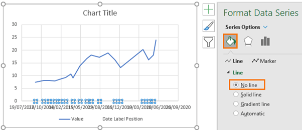
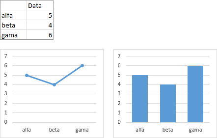
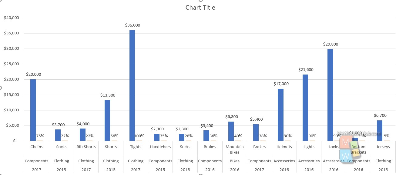
Hide zero value data labels for excel charts (with category name) Hide zero value data labels for excel charts (with category name) I'm trying to hide data labels for an excel chart if the value for a category is zero. I already formatted it with a custom data label format with #%;;; As you can see the data label for C4 and C5 is still visible, but I just need the category name if there is a value. › documents › excelHow to hide zero data labels in chart in Excel? - ExtendOffice Note: In Excel 2013, you can right click the any data label and select Format Data Labels to open the Format Data Labels pane; then click Number to expand its option; next click the Category box and select the Custom from the drop down list, and type #"" into the Format Code text box, and click the Add button. How to hide points on the chart axis - Microsoft Excel 2016 Excel 2016. Sometimes you need to omit some points of the chart axis, e.g., the zero point. This tip will show you how to hide specific points on the chart axis using a custom label format. To hide some points in the Excel 2016 chart axis, do the following: 1. Right-click in the axis and choose Format Axis... in the popup menu: › which-chart-type-worksWhich Chart Type Works Best for Summarizing Time-Based Data ... Jul 16, 2022 · The rule of thumb is to avoid presenting too much data in one chart, regardless of the chart type you use. Best practices for designing column charts #1 Start the ‘Y’axis value at zero. When you do not start the ‘Y’ axis value of a chart at zero, the chart does not accurately reflect the size of the variables.
Highlight Max & Min Values in an Excel Line Chart - Xelplus ...
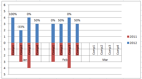
excel - Hide Category Name From bar Chart If Value Is Zero - Stack Overflow The data typically have some zero values in it that I do not want to show on the chart. I can hide the zero by using custom number format 0;"" but it still leaves the category name and the visible which makes the chart messy to read. Is there any way to accomplish this? enter image description here excel excel-charts Share asked May 3, 2021 at 6:30
Excel Waterfall Chart: How to Create One That Doesn't Suck
› excel › excel-chartsCreate a multi-level category chart in Excel - ExtendOffice 22. Now the new series is shown as scatter dots and displayed on the right side of the plot area. Select the dots, click the Chart Elements button, and then check the Data Labels box. 23. Right click the data labels and select Format Data Labels from the right-clicking menu. 24. In the Format Data Labels pane, please do as follows.
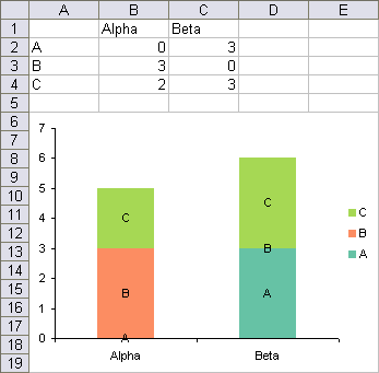
How-to Hide a Zero Pie Chart Slice or Stacked Column Chart ...
How to hide zero currency in Excel? - ExtendOffice To hide zero currency, you just need to add a semicolon ; after your cell formatting.. 1. Select the currency cells and right click to select Format Cells in the context menu.. 2. In Format Cells dialog, click Number > Custom, and then add ; at the end of the format you have set in the Type textbox.. 3. Click OK to close dialog. Now you can see the zero currency is hidden.

How to Use Cell Values for Excel Chart Labels
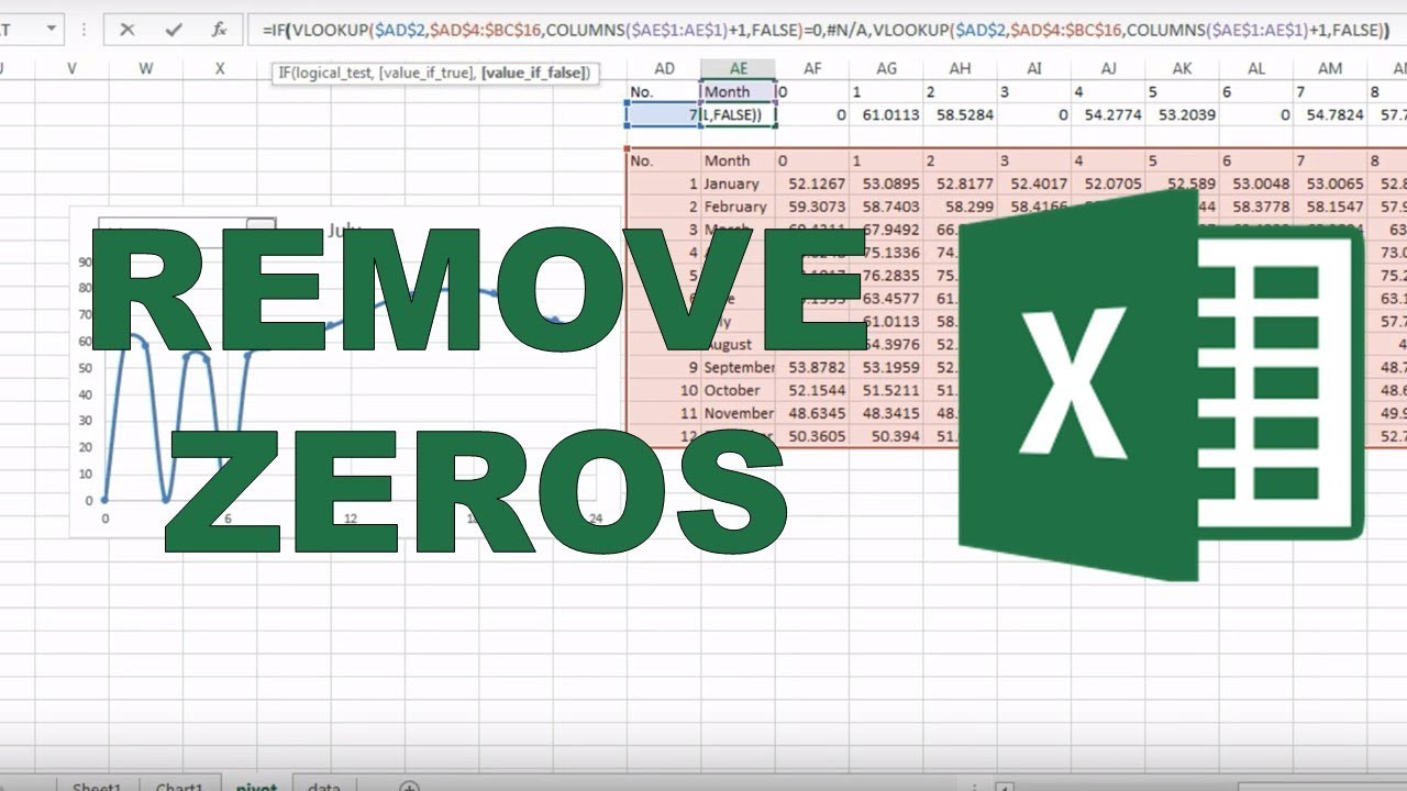
How to Quickly Remove Zero Data Labels in Excel - Medium In this article, I will walk through a quick and nifty "hack" in Excel to remove the unwanted labels in your data sets and visualizations without having to click on each one and delete ...

How to Change Excel Chart Data Labels to Custom Values?
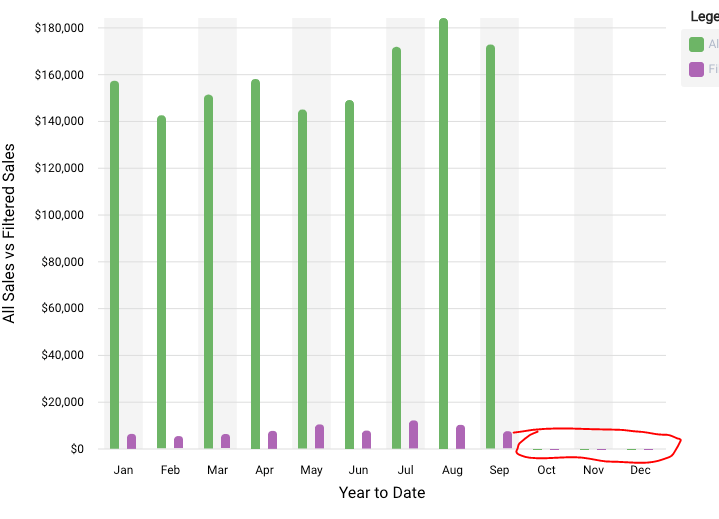
How to Hide Zero Data Labels in Excel Chart (4 Easy Ways) - ExcelDemy Now, we need to filter our dataset to hide the zero data labels in an Excel chart. First, select the range of cells B4 to C12. Then, go to the Data tab in the ribbon. After that, select Filter from the Sort & Filter group. It will filter our dataset. See the screenshot and you will see the filter drop-down option.
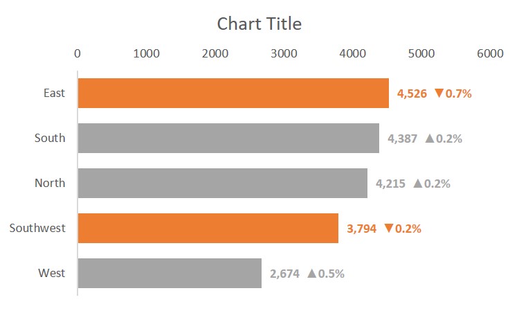
Add % Difference Data Labels to Excel Horizontal Tornado ...
› article › how-to-suppress-0How to suppress 0 values in an Excel chart | TechRepublic Jul 20, 2018 · The stacked bar and pie charts won’t chart the 0 values, but the pie chart will display the category labels (as you can see in Figure E). If this is a one-time charting task, just delete the ...
/simplexct/images/Fig2-79394.jpg)
How to Create a Bar Chart With Labels Above Bars in Excel
How to Hide Zero Values on an Excel Chart - YouTube

Hide zero values in Excel 2010 column chart - Microsoft Community
metacpan.org › pod › Spreadsheet::WriteExcelSpreadsheet::WriteExcel - Write to a cross-platform Excel ... Zip codes and ID numbers, for example, often start with a leading zero. If you write this data as a number then the leading zero(s) will be stripped. This is the also the default behaviour when you enter data manually in Excel. To get around this you can use one of three options. Write a formatted number, write the number as a string or use the ...

Remove Chart Data Labels With Specific Value
Hiding 0 value data labels in chart - Google Groups the worksheet, make sure you select the chart and take macro>vanishzerolabels>run. Sub VanishZeroLabels () For x = 1 To ActiveChart.SeriesCollection (1).Points.Count If ActiveChart.SeriesCollection...

Hide data labels when value is 0 (on pie graph) Excel2013 : r ...
Remove zero data labels on chart - Excel Help Forum If using formulas, include condition to exhibit #N/A instead of zero. Over chart area, right button options, click Select Data. At dialog box, click Hidden and blank cells. At new dialog box, click Show data in hidden rows and columns. Not sure about precise English version for those commands, but they will show something like that. Godspeed!
How to remove blank/ zero values from a graph in excel
Hide zero values in the data labels of a chart? - Ask LibreOffice I am using a line graph to display my spending over the course of a month, and I have chosen to display the data labels for added readability; however there are numerous days where my spending was zero and the "$0.00" being displayed at the bottom of the chart is mucking the readability up. Note; I do still want the data -point- to be there, I just want the -label- to go away for values=0 ...
How to Hide Zero Data Labels in Excel Chart (4 Easy Ways)
Add or remove data labels in a chart - support.microsoft.com On the Design tab, in the Chart Layouts group, click Add Chart Element, choose Data Labels, and then click None. Click a data label one time to select all data labels in a data series or two times to select just one data label that you want to delete, and then press DELETE. Right-click a data label, and then click Delete.

How to format axis labels individually in Excel
› documents › excelHow to add data labels from different column in an Excel chart? How to hide zero data labels in chart in Excel? Sometimes, you may add data labels in chart for making the data value more clearly and directly in Excel. But in some cases, there are zero data labels in the chart, and you may want to hide these zero data labels. Here I will tell you a quick way to hide the zero data labels in Excel at once.
Solved: bar chart suggestion to show zero values - Microsoft ...
Hide zero values in chart labels- Excel charts WITHOUT zeros ... - YouTube 00:00 Stop zeros from showing in chart labels00:32 Trick to hiding the zeros from chart labels (only non zeros will appear as a label)00:50 Change the number...
/simplexct/BlogPic-h7046.jpg)
How to Create a Bar Chart With Labels Above Bars in Excel
Change the format of data labels in a chart To get there, after adding your data labels, select the data label to format, and then click Chart Elements > Data Labels > More Options. To go to the appropriate area, click one of the four icons ( Fill & Line, Effects, Size & Properties ( Layout & Properties in Outlook or Word), or Label Options) shown here.

Google Workspace Updates: Get more control over chart data ...
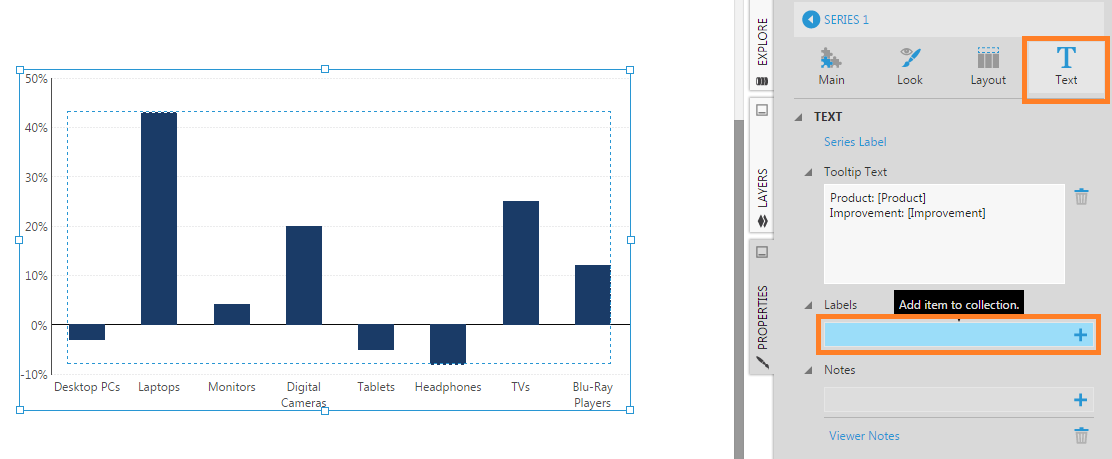
think-cell :: KB0195: How can I hide segment labels for If the chart is complex or the values will change in the future, an Excel data link (see Excel data links) can be used to automatically hide any labels when the value is zero ("0"). Open your data source Use cell references to read the source data and apply the Excel IF function to replace the value "0" by the text "Zero"
Excel bar chart with conditional formatting based on MoM ...
remove label with 0% in a pie chart. - social.msdn.microsoft.com Here is what I did: I wanted to remove the 0% percent labels from my pie chart that displays percentages next to each slice. Turn the range of cells that you want to make a pie chart with into a table. In excel 2007 you can do this by clicking Home>Format as Table>Select the Style You Want>Then Select the appropriate range.

microsoft excel - How to Hide Series Name Label, Call Out Box ...
Label Specific Excel Chart Axis Dates • My Online Training Hub
Aligning data point labels inside bars | How-To | Data ...
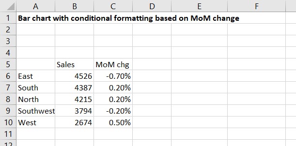
Excel bar chart with conditional formatting based on MoM ...

Display Customized Data Labels on Charts & Graphs
How to hide points on the chart axis - Microsoft Excel 365
How-to Easily Hide Zero and Blank Values from an Excel Pie ...

How can I hide 0% value in data labels in an Excel Bar Chart ...
Individually Formatted Category Axis Labels - Peltier Tech

Hide Zero Values In Data Labels - Excel Titan
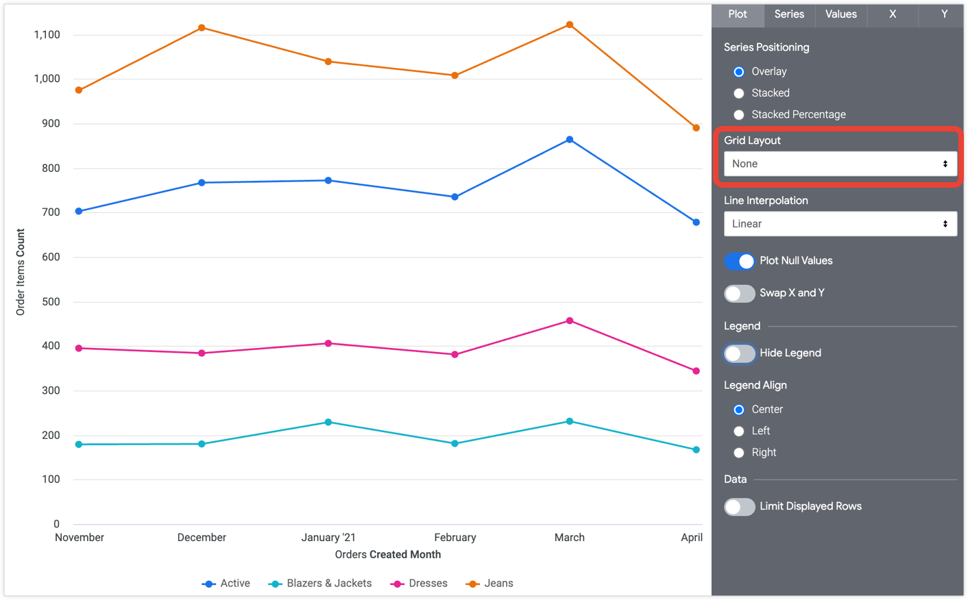
Line chart options | Looker | Google Cloud
Hide Series Data Label if Value is Zero - Peltier Tech
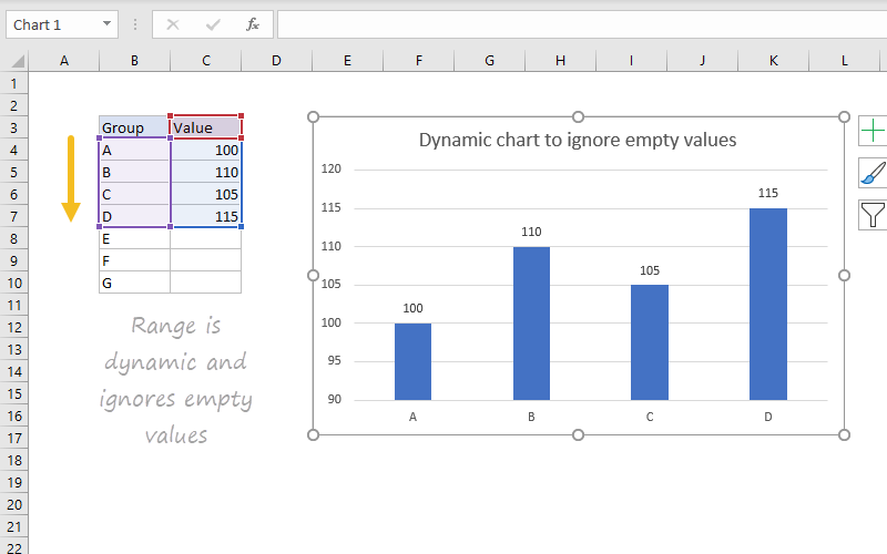
Column chart: Dynamic chart ignore empty values | Exceljet

7 Amazing Excel Custom Number Format Tricks (you Must know)
Excel How to Hide Zero Values in Chart Label - YouTube

Custom Data Labels with Colors and Symbols in Excel Charts ...
How to hide zero values in an Excel graph - Quora

Hide zero values in the data labels of a chart? - English ...
How to add or remove data labels with a click - Goodly
How To Show Or Hide Data Labels On MS Excel? | My Windows Hub
How to Create Waterfall Charts in Excel - Page 5 of 6 - Excel ...
How to hide Zero data label values in pie chart ssrs

Showing the Total Value in Stacked Column Chart in Power BI ...

KB0195: How can I hide segment labels for "0" values ...
libxlsxwriter: Working with Charts
Post a Comment for "42 excel chart hide zero data labels"